A tolerance stack up calculates the effects of accumulated variation allowed by specified engineering-drawing dimensions and tolerances to determine the maximum and minimum distance, whether clearance or interference, between two features or parts. Worst-case (arithmetic, deterministic, or high-low) tolerance analysis places every contributor at its specified tolerance limit to guarantee 100 percent assembly and interchangeability when inspected parts stay inside their intervals, whereas statistical root sum square (RSS) analysis models independent, centered component distributions to trade 100 percent interchangeability for looser part tolerances and lower fabrication costs.
Within our DFM and hardware engineering guides and all engineering articles, this guide covers one-dimensional clearance-chain setup, vector-loop sign rules, worst-case versus RSS formulas, and worked numerical comparisons. Broad milestone deliverables stay in what is design for manufacturing, BOM part-count reduction rules stay in design for manufacturing and assembly, supplier Fit-and-Draft review discussions stay in mechanical design engineer DFM handover skills, and release package file audits stay in the manufacturing specification handoff checklist.
| Analysis dimension | Worst-case (arithmetic / high-low) analysis | Statistical root-sum-square (RSS) analysis |
|---|---|---|
| Core variation model | Places individual variables at their tolerance limits to make the assembly measurement as large or as small as possible, ignoring the distribution inside those limits. | Models each component variation as a statistical distribution and sums independent distributions to predict the assembly variation distribution rather than extreme limits. |
| Assembly tolerance formula (|ai| = 1) | Tassy arith = T1 + T2 + … + Tn, accumulating linearly with the number of parts n. | Square root of the sum of squared detail tolerances, accumulating as the square root of the number of parts when the mean equals the nominal dimension. |
| Conformance and interchangeability | Guarantees 100 percent fit with mathematical certainty if parts are inspected so |Li − λi| ≤ Ti holds for every detail. | Abandons 100 percent interchangeability; predicts a .9973 (99.73 percent) assembly compliance probability and .27 percent failure share under centered Gaussian Ti = 3σi assumptions. |
| Effect on component tolerances | Often requires very tight individual component tolerances, leading to expensive manufacturing and inspection processes and/or high scrap rates. | Yields part tolerances that are much more liberal than those obtained under arithmetic tolerancing when contributors are independent and centered. |
| Primary selection boundary | Used when arithmetic results already meet the gap limit, or when required by customers for critical mechanical interfaces and spare part replacement interfaces. | Used in mass production when worst-case tolerancing is not a contract requirement and contributors come from independent, centered processes with small sensitivities. |
What Is a Tolerance Stack Up in Mechanical Design?
In mechanical engineering, tolerance analysis is the general term for activities related to studying accumulated variation in mechanical parts and assemblies, including 2D tolerance stacks, 3D Monte Carlo simulations, and datum conversions. An engineering tolerance sets the permissible limit or limits of variation in a physical dimension or in the space between mating features such as a bolt and a nut or a hole; a variation beyond that tolerance is noncompliant, rejected, or exceeding the tolerance.
In mass production rather than custom-made fabrication, exact dimensions paired with controlled tolerances enable interchangeable parts: components made to specifications so nearly identical for practical purposes that one part can freely replace another in any assembly of the same type without custom fitting such as filing. As defined in the U.S. Department of Commerce May 2000 tolerance analysis report, tolerance synthesis allocates tolerances among component geometric parameters to minimize tolerance-driven cost while satisfying functional and assembly requirements, whereas tolerance analysis evaluates the aggregate behavior of individual tolerances on a measurable assembly response Y such as an assembly gap.
While no official engineering standard covers the process or format of tolerance analysis and stackups, the stackup methods depend somewhat upon the dimensioning and tolerancing standards referenced on the engineering drawing, such as American Society of Mechanical Engineers (ASME) Y14.5, ASME Y14.41, or relevant ISO dimensioning and tolerancing standards. Designers conducting tolerance stack up analysis rely on two fundamentally different tools: worst case tolerance analysis (also called deterministic or high-low tolerance analysis), which provides a conservative benchmark, and statistical analysis (such as RSS or Monte Carlo), which provides an optimistic benchmark.
How Do You Build a Vector Loop for a 1D Clearance Chain?
A one-dimensional tolerance loop starts at one side of an intended gap after pushing the parts in the assembly to one side or another of their loose range of motion. Contributing dimensions are drawn as vectors joined tip-to-tail, forming a tolerance path or tolerance chain that passes through each part in the assembly in succession.
When tracing a vector loop through an individual part and across joints, follow four sequential steps:
- Enter the part through a joint.
- Follow the datum path to the datum reference frame (DRF).
- Follow a second datum path leading to another joint.
- Exit to the next adjacent part in the assembly.
Loops must pass through every part and every joint in the assembly. A single vector loop may not pass through the same part or the same joint twice, though it may start and end in the same part. If a vector loop includes the exact same dimension twice in opposite directions, that dimension is redundant and must be omitted. While general kinematic assemblies require one loop for each three kinematic variables (joint degrees of freedom), those modeling rules vary depending on whether a 1D, 2D, or 3D tolerance stackup method is used.
The Cogwheel Case Clearance Chain (n = 6)
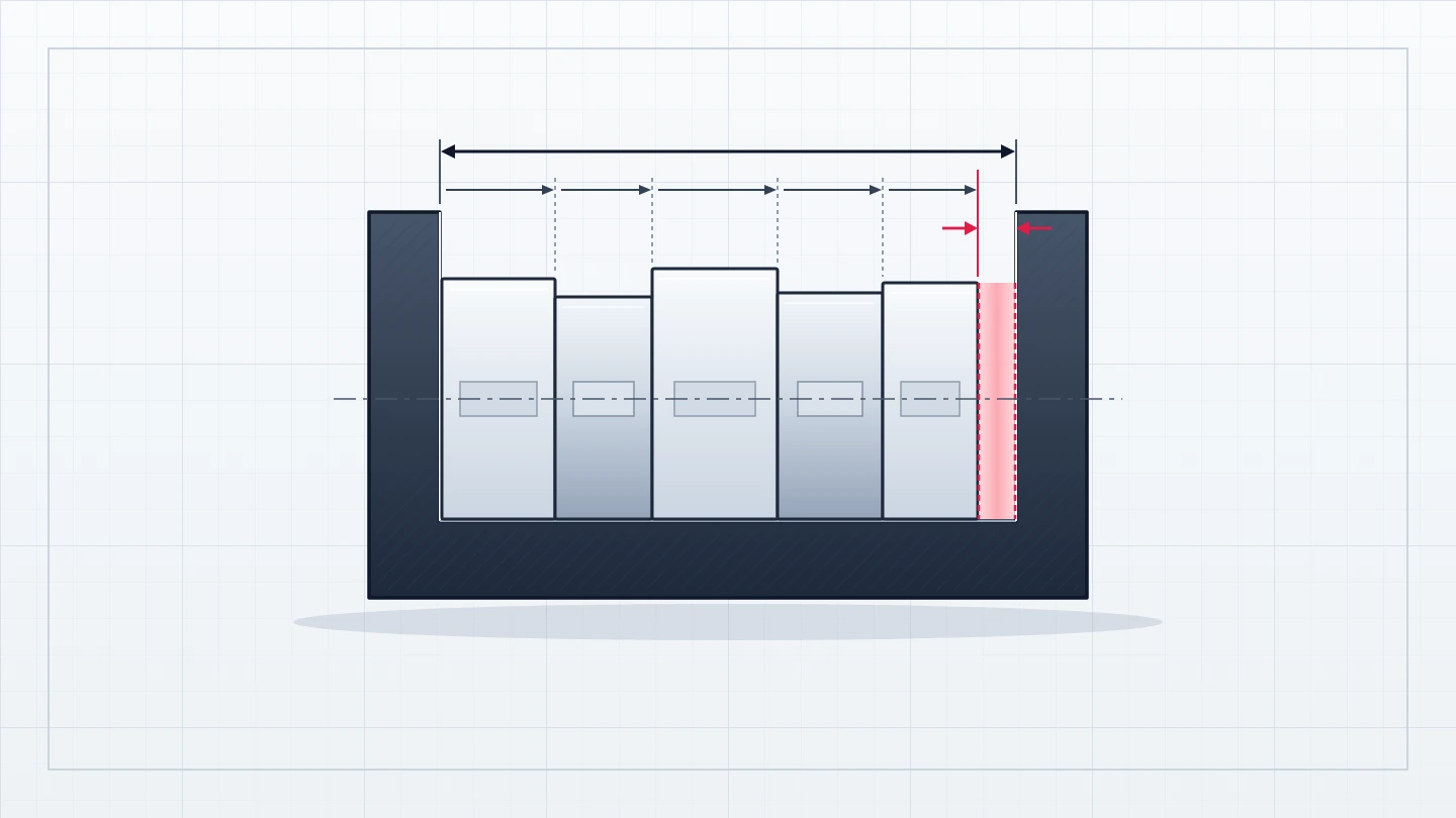
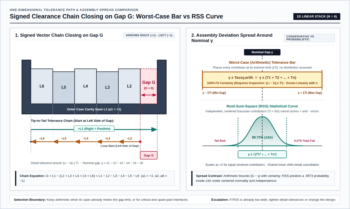
In Fritz Scholz’s technical report on tolerance stack analysis methods, a stack of cogwheels inside a case illustrates how a one-dimensional clearance chain assigns signs to six lengths (n = 6). The outer case cavity length is L1, and the five stacked internal lengths are L2, L3, L4, L5, and L6; the remaining gap needed for L2 to butt up to L1 is the assembly clearance gap G:
G = L1 − (L2 + L3 + L4 + L5 + L6) = L1 − L2 − L3 − L4 − L5 − L6
For proper assembly it is desired to have G > 0, and for functional performance reasons a designer may also limit G from above. On the horizontal chain diagram, arrows point right for positive contributions and left for negative ones, giving sign coefficients a1 = 1 and a2 = … = a6 = −1 (where each coefficient ai in a length chain is either +1 or −1). Evaluating the nominal part dimensions with the same signs gives the nominal gap γ = λ1 − λ2 − λ3 − λ4 − λ5 − λ6, while each detail tolerance Ti represents an upper limit on the absolute deviation between actual length Li and nominal length λi, written |Li − λi| ≤ Ti.
Worst-Case vs RSS Formulas and Statistical Assumptions
Worst-case analysis and statistical RSS analysis start from the same linear gap equation and differ in how they interpret the detail tolerance bound |Li − λi| ≤ Ti.
Worst-Case Tolerance Analysis Formula
Arithmetic tolerance stackups bound the assembly gap deviation |G − γ| by summing the absolute weighted tolerances:
Tassy arith = |a1|T1 + |a2|T2 + … + |an|Tn
When |ai| = 1 for all i = 1, …, n, the worst-case assembly tolerance simplifies to the direct sum Tassy arith = T1 + T2 + … + Tn. As noted in Scholz’s critical review of tolerance stack methods, the validity of this bound hinges solely on every detail satisfying |Li − λi| ≤ Ti regardless of the statistical distribution inside each interval. If every part dimension lies inside its specified interval and Tassy arith satisfies the assembly requirement, every assembly fits with mathematical certainty; without inspection to verify |Li − λi| ≤ Ti, there is no 100 percent guarantee of assembly.
Because worst-case errors accumulate linearly with the number of parts n, reverse tolerance allocation tightens rapidly as part count rises. In Scholz’s critical review, if proper assembly requires an arithmetic stack tolerance TAarith ≤ QA = .00400 across n equal contributors, each common part tolerance has to satisfy T = TAarith / n ≤ .00400 / n.
Root-Sum-Square (RSS) Formula and Three Core Assumptions
In statistical error propagation, Walla Walla University’s error-accumulation lecture notes state that random zero-mean errors between tolerance limits accumulate as sqrt(N) when the mean equals the nominal dimension, because positive and negative errors cancel. For a linear chain where ai = ±1 for all i = 1, …, n, the Root Sum of Squares (RSS) assembly tolerance equals the square root of the sum of the squared detail tolerances, producing part tolerances that are much more liberal than those obtained under arithmetic tolerancing.
In Scholz’s critical review, when the assembly criterion A is Gaussian, 99.73 percent of all assembly values fall within ±3σA = ±TARSS of the nominal value νA, meaning .27 percent of assemblies fail. That .9973 probability depends on three explicit assumptions:
- A Gaussian (normal) density fi for the variation.
- A part-dimension process centered on the nominal value (νi = µi).
- Detail tolerance set to three standard deviations (Ti = 3σi), so 99.73 percent of individual Li values fall within the tolerance interval.
Three is not the only sigma factor used in the literature: Mansoor (1963) appears to prefer the factor 3.09, corresponding to a .999 probability for individual part tolerance compliance. Regarding normality, the May 2000 NIST report notes that for linear, mutually independent gap measures, normal individual distributions make the assembly response Y normally distributed, and even when individual distributions are not normal, Y can be treated as normal by invoking the central limit theorem. Scholz’s Spring Quarter 2007 STAT 498 B notes likewise state that the normality assumption is a simplification and is not essential, while his tolerance-stack report calls the independence assumption probably the most essential cornerstone of statistical tolerancing because it allows some cancellation of variation from nominal.
Worked Example: Ten-Disk Stack Under Worst-Case vs RSS
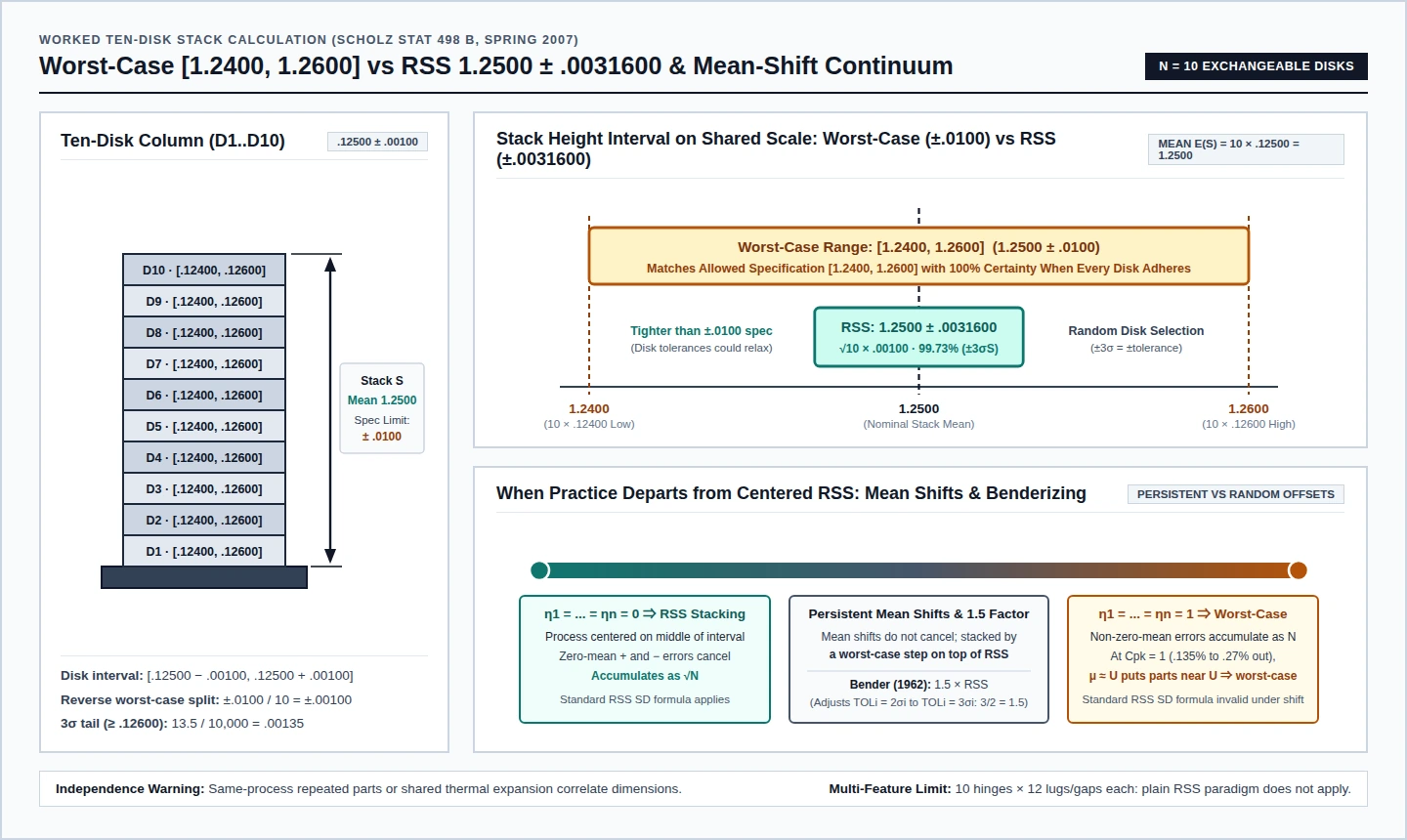
Scholz’s Spring Quarter 2007 STAT 498 B notes compare arithmetic worst-case tolerancing and RSS on a stack of ten exchangeable disks, using typical two-sided specifications of the form [Nominal − Tolerance, Nominal + Tolerance] (noting that specifications can also be one-sided).
Each individual disk is specified within [.12500 − .00100, .12500 + .00100] = [.12400, .12600], and the stack of ten disks should be 1.2500 high with ± .0100 tolerance, giving an allowed stack height range of [1.2500 − .0100, 1.2500 + .0100] = [1.2400, 1.2600].
Under worst-case (arithmetic) tolerancing, adhering to the single-disk interval guarantees the ten-disk stack specification: ten disks at .12600 produce the highest stack of 10 × .12600 = 1.2600, and ten disks at .12400 produce the lowest stack of 10 × .12400 = 1.2400, matching the total possible range [1.2400, 1.2600]. Reversing that end tolerance across the ten disks assigns ±.0100 / 10 = ±.00100 to each individual disk, illustrating how end tolerances can create very tight, unrealistic, costly item tolerances.
Under statistical tolerancing, disks are chosen at random rather than arranged deliberately into a worst possible stack. Setting ±3 standard deviations equal to ± tolerance puts 13.5 out of 10,000 disks at or above .12600, so the chance of randomly selecting one disk that thick or thicker is .00135 = 13.5 / 10,000. With each disk centered on .12500, the mean stack height is E(S) = E(D1) + … + E(D10) = 10 × .12500 = 1.2500, and the RSS method gives a three-sigma stack interval (µS ± 3σS, containing 99.73 percent of normal S values) of:
1.2500 ± .0031600, where .0031600 = √10 × .00100
Because ±.0031600 is much tighter than the ±.0100 stack specification, the designer could consider relaxing the individual disk tolerances.
| Ten-disk stack metric (STAT 498 B example) | Worst-case (arithmetic) calculation | Centered independent RSS calculation |
|---|---|---|
| Individual disk specification | [.12500 − .00100, .12500 + .00100] = [.12400, .12600] | Random selection with ±3 standard deviations = ±.00100 tolerance (13.5 / 10,000 = .00135 ≥ .12600) |
| Stack mean and tolerance half-width | Nominal 1.2500 with ±.0100 half-width | Mean E(S) = 10 × .12500 = 1.2500 with ±.0031600 half-width (√10 × .00100) |
| Predicted stack height interval | [1.2400, 1.2600] from 10 × .12400 to 10 × .12600 (100 percent guarantee if adhered to) | 1.2500 ± .0031600 containing 99.73 percent of normal stack values (µS ± 3σS) |
| Implication for disk tolerances | Reverse allocation forces ±.0100 / 10 = ±.00100 per disk | Stack spread sits well inside ±.0100, so individual disk tolerances could be relaxed |
When Does RSS Fail, and How Do Mean Shifts or Benderizing Adjust It?
Practice has shown that arithmetic tolerancing tends to give overly conservative results while the basic RSS method is often too optimistic. Several physical and statistical conditions break plain RSS cancellation and govern method selection:
- Correlated processes and thermal changes: Independence is reasonable when part dimensions come from different manufacturing or machining processes, whereas several similar or identical parts from the same process in one assembly or thermal expansion affecting parts similarly undermine independence.
- Persistent mean shifts and a Cpk of 1: Sums of non-zero-mean errors accumulate linearly as N without cancellation, such as when an operator stops material removal as soon as a part enters the tolerance zone. In NIST’s Motorola subsection, standard RSS formulas apply when there is no mean shift, and in the presence of a mean shift the standard RSS formula cannot be used for computing the standard deviation of Y. Because mean shifts represent persistent effects that do not play out independently for each part, Scholz’s STAT 498 B notes stack mean shifts in a worst-case step: zero mean-shift ratios (η1 = … = ηn = 0) return RSS stacking, whereas unit mean-shift ratios (η1 = … = ηn = 1) return worst-case arithmetical stacking. Even Cpk = 1 leaves between .135 percent and .27 percent of part dimensions out of tolerance and permits a process mean near the upper limit (µ ≈ U), which produces worst-case stacking.
- Benderizing (Bender, 1962): To counter optimistic RSS buildup, Bender (1962) proposed multiplying the RSS expression by 1.5 (3/2 = 1.5) to adjust experience-based tolerances from TOLi = 2σi to TOLi = 3σi.
- Nonlinearity and multi-feature exchangeability: Statistical error propagation is useful when errors and system sensitivities are small; if the assembly response function Y is highly nonlinear, applying RSS can lead to serious errors. Scholz’s report gives an example function that lacks derivatives at (0, 0), whose graph in 3-space looks like an upside cone with its tip at (0, 0, 0) and admits no tangent there, and his STAT 498 B notes show an assembly of 10 hinges with 12 lugs or gaps each where the RSS paradigm does not work.
- Decision boundaries when sizing a stack: If arithmetic stacking already gives satisfactory assembly tolerance results, there is little motivation to try other methods except possibly to relax detail tolerances. Conversely, if the RSS method does not give satisfactory assembly tolerance results, none of the other methods will make matters better, leaving only tighter detail tolerances or, if that is not feasible, a design change.
Spreadsheet Stack-Up Inputs, Simulation Methods, and Physical Limits
When organizing a one-dimensional stack-up calculation table, record the nominal dimensions λi and tolerances Ti from the engineering drawing, the chain sign coefficient ai (+1 or −1) from the tip-to-tail vector loop, and the functional gap requirement (such as G > 0, an upper functional limit, or an allowed arithmetic bound QA such as .00400). Compute Tassy arith alongside the RSS value, record the Gaussian, centered-mean, independence, and sigma-factor assumptions beside the RSS estimate, and keep any persistent mean-shift step separate from random zero-mean variation.
When moving beyond a linear 1D equation, NIST groups statistical propagation into four classes: linear stack tolerancing (RSS), nonlinear propagation via extended Taylor series, numerical integration (quadrature technique), and Monte Carlo simulation. Within statistical analysis tools, Wikipedia contrasts two chief modeling approaches:
| Statistical modeling approach | How assembly variation is computed | Primary analytical trade-off |
|---|---|---|
| Geometric-multiplier sensitivity method | Generates geometric multipliers by making small deltas to the nominal dimensions. | Output is smooth, yet it fails to account for geometric misalignment allowed by tolerances (assuming two parallel surfaces under a size dimension remain parallel even though the tolerance does not require this). |
| Random-geometry assembly simulation | Simulates variations through random geometry changes constrained by expected distributions within allowed tolerances, assembles the parts, and records critical measurements. | Captures acceptable imperfect geometry and can incorporate actual factory inspection data to test proposed changes, yet each run is unique so the output distribution and mean vary from run to run. |
Finally, a rigid dimensional sum does not capture every shop-floor risk. Designs often include a safety factor because of operational temperature and pressure of the parts or assembly, wear, deflection of components after assembly, and the possibility or probability that parts are slightly out of specification despite passing inspection. Writing a good set of engineering tolerances in a specification does not by itself achieve compliance: with a normal distribution, measured tails may extend well beyond plus and minus three standard deviations from the process average, so process capability needs to be compatible with the specified tolerances and process controls must be in place, and designers should remember Genichi Taguchi’s warning that treating two-sided tolerances like football “goal posts” implies that all values inside the limits are equally acceptable.